On this page
Predict. Change one thing. Measure.
These experiments use the default virtual platform and its ideal actuators, not a commercial device. Use the named classic preset between experiments; from Ball Lab first choose Exit to platform workbench. Times below are simulated time, not a promise of real-time performance. Millimetres are displayed in the UI; the solver uses metres, radians, kilograms, seconds and newtons.
1. Make it move, then solve it backwards
Question: Can six leg lengths describe a table that both moves and tilts?
Open the IK lesson, or choose Move in the classic experiment bar. In Control, set X=25 mm, Y=−15 mm, Z=575 mm, Roll=4°, Pitch=−3°, Yaw=5°. Changing a pose field stops the automatic trajectory. Leave the six sliders active and gravity compensation on.
Watch the dashed target outline, actual table and error readouts. The errors should settle toward zero under these moderate gains. Different legs extend by different amounts; tilting is not simply changing all lengths together.
Now select IK · FK → Copy target lengths → Solve forward kinematics. Read the residual and reconstructed pose. Click Apply solution as control target. This changes the target, not the physical state.
Explain it: IK is geometry from pose to lengths. FK is a local numerical reconstruction in the opposite direction. A small FK residual says those lengths fit that computed pose; it is not a uniqueness proof or a collision check. Theory §§1–2.
Challenge: Solve from the home seed and previous solution. Why might a distant or invalid set of lengths fail? Do not treat a solver failure as a usable pose.
2. Measure a virtual spring
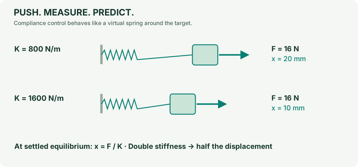
Question: How far should a 16 N force move a spring of stiffness 800 N/m?
Choose Push in the classic experiment bar, or open the compliance lesson. This resets the mechanism, selects Compliance, sets translation K=800 N/m and applies sustained +X force of 16 N. Wait about 1.5 simulated seconds. X should approach 20 mm in this default case.
spring force = stiffness × displacement
F = K x
x = F / K = 16 / 800 = 0.020 m = 20 mm
Open Dynamics → Release all forces. Wait another 1.5 simulated seconds and watch it return near the target. This is an active controller acting like a spring, not a physical spring added to every joint. The separate Push plate button applies an impulse of 2 N·s; it is not the same load.
Change one thing: Repeat with K=1600 N/m and predict 10 mm. Then vary translation D while keeping K fixed. D changes the transient response; in this simple steady-state case it does not set the final F/K displacement.
Record: Save project and CSV. At least record applied force, K, D, elapsed simulation time, final X, saturation count and allocation residual.
Boundary: F/K is an equilibrium estimate for the unsaturated, sufficiently actuated default system with gravity compensation and without added passive stiffness or contact. It is not a universal six-dimensional law for every configuration. The implementation is direct task-space impedance control, not a separate force-sensor-driven admittance controller. Theory §5, Hogan.
3. Hold the weight without holding a position
Question: Is cancelling weight the same as moving to a target?
Choose Gravity in the classic experiment bar, or open the gravity lesson. At rest, the same-model feedforward effort nearly balances the modelled weight. There is no position PD in this mode; modest joint damping remains.
Click Push plate. The platform can move because gravity compensation does not create a position-restoring spring. Reset and choose Drives off: now the active motor commands are zero and gravity lowers the platform until other model forces, such as a stop, act.
Explain it: An elevator can have a motor force that balances its weight without knowing which floor you want. Position control additionally needs a target and feedback.
Challenge: In Design, change payload mass, apply geometry, then select Control → Gravity compensation (not the resetting preset). Both the controller and plant know the edited mass in this lab. Their agreement does not test robustness to an unknown real payload. A meaningful robustness study would deliberately separate estimated and actual parameters; that feature is not provided here.
4. Turn a motor into a passive connection
Question: Can a connection support weight without an active motor?
Choose Passive in the classic experiment bar, or open the passive lesson. All six sliders are passive; default springs and dampers support the platform with some sag. In Joints, select P1 and inspect its k/c. Use Capture all rests only deliberately: this changes the unstrained reference and can change stored energy instantaneously.
For a controlled comparison, reset, pause, choose 6P passive, and set the same k/c on all six sliders. Run and record the height. Increase stiffness on all six; compare the sag. Change damping; compare how quickly oscillations settle. Changing only P1 also makes the support asymmetric and can tilt the table.
Now examine B1 or T1. These are spherical joints with three rotational axes. Their k/c units are N·m/rad and N·m·s/rad, not N/m. Active spherical actuation is an ideal mathematical three-axis torque model, not an assertion that a standard ball joint contains three motors.
Important: With only one linear motor disabled, arbitrary six-axis force demands may no longer be achievable. Inspect the allocation residual instead of assuming the platform can still follow every target. Passive ≠ locked and active ≠ unlimited force.
For teachers and researchers
A 20-minute session can use experiment 1 for prediction, experiment 2 for a measurement table, and a final discussion of one missing physical effect. No learner needs to edit code. A longer session can derive the leg Jacobian and compare numerical and analytic derivatives.
Undergraduate extension: derive l_dot = J [v; omega] and use power balance to justify W = J^T f for this lab's Jacobian convention. Graduate extension: inspect the leg-spin coordinates, gravity potential gradient, positive-definite mass matrix and the contact-free energy identity in the regression tests. Repeat at smaller timesteps before making an integration-accuracy claim.